Saturday 16 December 2017

Lab 6: Static Corrections

INTRODUCTION 
Static corrections are applied to seismic data in order to compensate for various effects on the data such as those related to near surface, variations in elevations, weathering and reference to a datum.


OBJECTIVE:

  • ·     To apply static correction to the stacked data.
  •       To adjust seismic traces in such a way that sources and receivers are present at one horizontal level.

PROCEDURE:

      1.     The NMO corrected seismic data and its header is loaded.
      2.     Static correction is applied.
      3.     The static corrected data is stacked.
      4.     Stacked data is loaded again.
      5.     Stacked and the static corrected stacked data is displaye

...load SeismicData_gain_bpf_sdecon_gain_sorted_nmo_corrected_stacked_A.mat cmp_num t Dstacked
%%
cmp_start=205;
cmp_end=205;
lags=20;
Dsort_static=scr_static(Dsort,Hsort,cmp_start,cmp_end,lags);
[Dstacked_static,t,cmp_num]=sstack(Dsort_static,Hsort);
%%
save SeismicData_gain_bpf_sdecon_gain_sorted_nmo_corrected_static Dsort Dsort_static Hsort Dstacked_static cmp_num t
%%

% Display Colored scale
scale=1;
figure(1);
simage_display(Dstacked,cmp_num,t,1)
xlabel(['CMP:',num2str(cmp_num),''],'FontSize',14)
ylabel('Time(s)','FontSize',14)
title ('Before Static Correction','FontSize',14)

% Display Colored scale
scale=1;
figure(2);
simage_display(Dstacked_static,cmp_num,t,1)
xlabel(['CMP:',num2str(cmp_num),''],'FontSize',14)
ylabel('Time(s)','FontSize',14)
title ('After Static Correction','FontSize',14)


..RESULTS 

DISCUSSION:

Both Figures are showing the stacked data before and after conducting the static correction. there are same  differences between these two figures. first Figure  is the original data. After applying the static corrections, the seismic section is getting better since the noise has been attenuated a bit and the background is much smoother than before as seen in second Figure due to  the elevation between sources and receivers has been corrected.


CONCLUSION:

Static corrections are applied to seismic data in order to compensate various effects on the data itself. There are two types of static corrections. The first type is the elevation static correction where it accounts for variable elevations of the sources and receivers meanwhile the second type is the residual static correction where it accounts for lateral variations in the velocity and thickness of the rock layers. Since the elevation between the sources and receivers are not in the vertical alignment, it causes some changes in travel time. By conducting the static correction, it will correct the alignment between these sources and receivers so that the seismic section will show a smoother result at the end of the analysis.

Lab 5: Sorting, Velocity Analysis and Stacking

INTRODUCTION 

Common Midpoint Sorting
Surface seismic reflection surveys are commonly acquired using the common midpoint (CMP) method. In this method, points in the subsurface are covered more than once by primary reflections from different source-receiver pairs.  Other names for this method include common reflection point (CRP) and common depth point (CDP). Traces reflected from the same midpoint form a CMP gather while the number of traces in a gather is called the fold of that gather. Common CMP folds are 80, 120, 240, and 480. Here the CMP spacing is half of the trace (receiver) spacing in a survey. 
Seismic data is acquired in the shot gather mode while most seismic data processing is performed in the CMP-offset mode. Therefore, we need to sort the traces between these modes. Generally, we need a way to sort the traces into other modes as well .

For this purpose, we use stacking charts in this lab . A stacking chart is a chart in which the x-axis indicates the geophone location and the y-axis indicates the source location. It is used to sort the traces into various modes or gathers such as shot, receiver, offset, or CMP. On a stacking chart (refer to Figure 5.3 which shows the data stacking chart):
 • Points along one diagonal have a common midpoint (the gather is called a common midpoint (CMP) gather). 
• Points along the other diagonal have a common offset (the gather is called a common offset gather (COG)). 
• Points along a horizontal line have a common source (the gather is called a common source gather).
 • Points along a vertical line have a common receiver (the gather is called a common receiver gather (CRG)).

Velocity Analysis
The velocity analysis is basically to determine the seismic velocities of layers in the subsurface. Many processing and interpretation stages such as: spherical divergence correction, NMO correction and stacking, interval velocity determination, migration and time to depth conversion uses the seismic velocities. There are different types of seismic velocities such as NMO, stacking, RMS, average interval, phase, group, and migration velocities. NMO, RMS and stacking velocities are the velocities that can be derived reliably from the time-space data
Normal moveout 
(NMO) describes the effect that the distance between a seismic source and a receiver (the offset) has on the arrival time of a reflection in the form of an increase of time with offset.The relationship between arrival time and offset is hyperbolic and it is the principal criterion that a geophysicist uses to decide whether an event is a reflection or not.It is distinguished from dip moveout (DMO), the systematic change in arrival time due to a dipping layer.
The normal moveout depends on complex combination of factors including the velocity above the reflector, offset, dip of the reflector and the source receiver azimuth in relation to the dip of the reflector


Objective:

To sort the shot gathered data into CMP, picking appropriate stacking velocities and stacking all CMPs in order to reveal a true image of the subsurface.

Practical
load SeismicData_gain_bpf_sdecon_gain.mat
[Dsort,Hsort]=ssort(Ds_gain,H);
save SeismicData_gain_bpf_sdecon_gain_sorted.mat Dsort Hsort
%% CMD sorting
[cmps,fold_cmp]=extracting_cmp_fold_num(Dsort,Hsort);
figure,stem(cmps,fold_cmp,'-')
xlabel('CMP numbers','FontSize',14)
ylabel('Fold','FontSize',14)
set(gca,'YMinorGrid','on')
%%
cmp_num=250;
[Dcmp,dt,t,cdp,jj,cmp_offset]=extracting_cmp(Dsort,Hsort,cmp_num);
scale=2;
mwigb(Dcmp,scale,cdp,t)
xlabel(['CMP:',num2str(cmp_num),''],'FontSize',14)
ylabel('Time(s)','FontSize',14)

clear all,close all,clc
load SeismicData_gain_bpf_sdecon_gain_sorted_A.mat
%%
cmp_step=5;
cmp_start=205;
cmp_end=255;
vmin=5000;
dv=200;
nv=51;
n_pts=8;
%% Velocity picking
[v_stack,t_stack]=vel_picking(Dsort,Hsort,vmin,dv,nv,cmp_start,cmp_end,cmp_step,n_pts);
%% save
save SeismicData_gain_bpf_sdecon_gain_sorted_velocities_A.mat v_stack t_stack cmp_step cmp_start cmp_end


RESULTS:
Wiggle trace shot gather 250 


Velocity +1500ms with NMO correction


Velocity -1500ms with NMO correction

DISCUSSION:
The first figure is the wiggle trace shot gather. After doing the sorting to CMP gathers, velocity analysis and stacking, it can be seen in these six figures (add subtract 1400ft/s) that the data are less chaotic and it starts to show the real image of a subsurface data. NMO correction is also done along the processes after the seismic velocity of layers has been determined, before stacking.


CONCLUSION:
  • ·       All objectives are achieved.
  •       This lab has shown almost the true figure of the subsurface geology.

Lab 4: Seismic Deconvolution

1. INTRODUCTION 
Deconvolution is a filtering process which removes a wavelet from the recorded seismic trace by reversing the process of convolution. The commonest way to perform deconvolution is to design a Wiener filter to transform one wavelet into another wavelet in a least-squares sense. By far the most important application is predictive deconvolution in which a repeating signal (e.g. primaries and multiples) is shaped to one which doesn't repeat (primaries only). Predictive deconvolution suppresses multiple reflections and optionally alters the spectrum of the input data to increase resolution. It is almost always applied at least once to marine seismic data.

OBJECTIVES:
  • ·       To increase the vertical resolution of the data by compressing the source wavelet
  • ·       To extract the useful information from the header using MATLAB function
  • ·       For noise attenuation of the seismic data
  • PROCEDURE:
clear,clc,close all
load SeismicDataA_gain
%%
shot_num=4:6;
p=1;
[Dshot,dt,dx,t,offset]=extracting_shots(Dbpf,H,shot_num,p);
[nt,nx]=size(Dshot);
%%
scale=5;
mwigb(Dshot,scale,offset,t)
xlabel('Trace number','FontSize',14)
ylabel('Time(s)','FontSize',14)
%%
max_lag=0.2;
[Dauto,lags]=auto_correlation_map(Dshot,max_lag,dt);
scale=5;
mwigb(Dauto,scale,offset,lags)
xlabel('Trace number','FontSize',14)
ylabel('Time lag(s)','FontSize',14)
title('Auto_correlograms of shot gathers 4-6','FontSize',14)
%%
mu=0.1;
Ds=spiking_decon(Dshot,max_lag,mu,dt);
scale=5;
mwigb(Dt,scale,offset,t)
xlabel('Trace number','FontSize',14)
ylabel('Time(s)','FontSize',14)


After applied frequency filtering via BPFs, the seismic data were smooth hence its vertical resolution affected due to the loss of some of original wider frequency band. The main objective  for seismic deconvolution is to increase the vertical resolution of the data by compressing the source wavelet to a zero phase if possible. 
This concept will be illustrated by using the spiking deconvolution as an example. The aim of spiking deconvolution is to compress the source wavelet w(t) into a zero-phase spike of zero width, i.e., δ(t). This means that we are eliminating the effect of the source wavelet and leave only the effect of the Earth’s reflectivity in the seismogram.By using M-function (provide in the manual) such as spiking_decon.m and auto_correlation_map.m to perform spiking deconvolution filtering.
both 
figure show that the shot gathers 4, 5 and 6 after apply the spiking deconvolution and instantaneous AGC with window length of 0.5 s to the deconvolved data which to compensate for the lost amplitude after deconvolution process.

Figure above showed the auto-correlograms for shot gather 4, 5 and 6. This auto-correlation window is important to choose the deconvolution parameters. The autocorrelation window should include the part of the record that contains useful reflection signal and should exclude coherent (e.g., ground roll) or incoherent noise (e.g., later parts of the record).

Figure above show the PSD of the average trace of shot gathers 4, 5 and 6 before and after using spiking deconvolution. From this figure we can conclude that the spiking deconvolution increase the frequency after apply the BPF (lab 3) which increase the vertical resolution.

DISCUSSION:
Deconvolution is done to increase the vertical resolution of the data. The deconvolution method specifically spiking deconvolution is conducted by compressing the source wavelet. Based on result  , it can be seen that the noise is reduced and the seismic data is much smoother. Thus, it is proved that spiking deconvolution does improve the seismic section.


CONCLUSION:
·       All objectives are achieved.
·       Spiking deconvolution is functioning in enhance the vertical resolution.


lab 3:Seismic Noise Attenuation

Introduction :
Why is noise attenuation important?
1- Very simply, removal of the noise allows for all other signal processes to work more effectively. Deterministic processes, such as deriving surface consistent amplitude corrections or deconvolution operators, rely heavily on the quality of the input data. Many summation processes related specifically to dual sensor 'OBC' processing require calibration of the amplitude levels of each component for successful summation. This calibration cannot be correct in the presence of excessive noise..
2-Removal of the noise is a key component in preparing the data for pre-stack imaging. Common Depth Point (CDP) stack is obviously one of the most effective noise attenuation tools but not an option with pre-stack imaging. The noise must be addressed prior to imaging
3-Properly addressing the noise provides the opportunity to track amplitude anomalies and stratagraphic objectives with confidence.
4-Effective noise removal, which preserves the original amplitude and phase characteristics of the data, provides the opportunity for advanced attribute work and inversion to better understand the reservoir.
Seismic data are highly corrupted with noise or unwanted energy arising from different kinds of sources. This unwanted energy can be classified into two main categories: 
 * Random noise (incoherent noise). 
*  Coherent noise.  
Seismic data processing, in general, can never eliminate all noise contaminating the data. Hence, the objective of seismic data processing is to improve as much as possible the signal-to-noise ratio (SNR). 

2. SEISMIC SIGNAL & NOISE 

Noise in seismic records is variable in both time and space. Poor seismic records usually have SNR ratios less than one. One can define the signal of interest (coherent energy) as the energy which is coherent from trace to trace. Random noise, on the other hand, is the energy that is incoherent from trace to trace. Furthermore, data from seismic events is correlated and its energy is generally concentrated in a fairly narrow band of, while noise is more uncorrelated and broadband. However, this is only true for random noise. Spatially coherent noise is the most troublesome noise and can be highly correlated and sometimes aliased with the signal and. In general, noise can be considered as anything other than the desired signal. A more proper definition of noise contaminating seismic signals can be stated by defining the type of signals we are interested in. The authors in define the signal of interest as the energy that is most coherent and desirable for geophysical interpretation of primarily reflected arrivals (signals). Anything other than that is considered to be unwanted energy, i.e., noise. 

2.1 RANDOM NOISE

Disturbances in seismic data which lack phase coherency between adjacent traces are considered to be random noise. Unlike coherent noise energy, such energy is usually not related to the source that generates the seismic signals. In land seismic records, near-surface scatterers, wind, rain, and instrument are examples of sources generating random noise. Based on the assumption that random noise is an additive white Gaussian noise (AWGN), it can be attenuated easily in several different ways such as frequency filtering, deconvolution, wavelet denoising, filtering using Gabor representation, stacking and many other methods. As discussed before in Chapter 1, stacking usually suppresses most of the incoherent noise and, therefore, improves the SNR by a factor of √M, where M is equal to the number of stacked traces. 

2.2 COHERENT NOISE 

 coherent noise is the energy which is generated by the source. It is an undesirable energy that is added to the primary signals. Such energy shows consistent phase from trace to trace. Examples of such a type in land seismic records are: multiple reflections or multiples, surface waves like ground roll and, air waves, coherent scattered waves, dynamite ghosts, etc. Improper removal of coherent noise can affect nearly all the processing techniques and complicates interpretation of geological structures. There exist loads of techniques which deal with the problem of suppressing / attenuating coherent noise 
that contaminates seismic data. Since our real seismic data contains mainly ground roll coherent noise, its main characteristics will be described in the following subsection. 


OBJECTIVES:
  • ·       To plot the magnitude spectra of shot gathers in frequency domain
  •      To apply finite impulse response (FIR) and infinite impulse response (IIR) filter on shot
         gathers
  •      To compare between the original data with applied filter data
PROCEDURE:
From this lab there were exist different means for such useful analysis: the frequency (or wave number) content of one-dimensional (1D) time (or space) signals, two-dimensional (2D) like the frequency-space (fx) or the frequency-wave number (fk) spectra; each of which can be used to obtain meaningful interpretation and, therefore, apply a suitable filtering technique. These plots and their corresponding analysis and interpretations are very useful, particularly, when applying linear filtering to 1D and/or 2D seismic data. You can use the following MATLAB m-file fx.m and fk.m (provided with the manual) to obtain the fand fmagnitude spectra in dB.

clear,clc,close all
load SeismicDataA_gain
%%
shot_num=8:18;
p=0;
[Dshot,dt,dx,t,offset]=extracting_shots(Dgz,H,shot_num,p);
%%
scale=2;
mwigb(Dshot,scale,offset,t)
xlabel('Offset(ft)','FontSize',14)
ylabel('Time(s)','FontSize',14)
%%
[Data_f,f]=fx(Dshot,dt);
figure,
pcolor(offset,f,20*log10(fftshift(abs(Data_f),1)))
shading interp;
axis ij;
colormap(jet)
colorbar
xlabel('Offset(ft)','FontSize',14)
ylabel('Frequency (Hz)','FontSize',14)
set(gca,'xaxislocation','top')
axis([min(offset),max(offset),0,max(f)])
%%
[Data_fk,f,kx]=fk(Dshot,dt,dx);
figure,
pcolor(kx,f,20*log10(fftshift(abs(Data_fk))))
shading interp;
axis ij;
colormap(jet)
colorbar
xlabel('Wavenumber(1/ft)','FontSize',14)
ylabel('Frequency(Hz)','FontSize',14)
set(gca,'xaxislocation','top')
axis([min(kx),max(kx),0,max(f)])
%%
N=100;
cut_off=[15,60];
[Dbpf,Dbpf_f]=bpf_fir(Dshot,dt,N,cut_off);
save SeismicDataA_gain


Figure above shows that shot gather 8 before and after applying the above mentioned BPF on each trace with the difference between both of them where clearly too great amount of the ground roll noise has been filtered


this figure also shows the f-x magnitude where the spectrum was banded between 15 and 60 Hz. Although frequency filtering like BFP has improved the data SNR by attenuating the ground roll noise, it has also lower the vertical resolution of the seismic data.

CONCLUSION:
  • ·       The objectives are achieved.
  •      High pass filter is useful to remove high frequency noise (ground roll).
  •        Band pass filter is useful to remove noise while preserving reflectors.


Friday 8 December 2017

Lab 2: Seismic Data QC

QUALITY CONTROL OF SEISMIC DATA

  Quality control (QC) has generally been considered by the seismic data acquisition industry to be a method to determine if the recording system is performing within the tolerances of the instrument manufacturer’s specifications and that the geophysical specifications of the survey design are being matched. 
With today’s modern recording systems there is a large amount of information that is being recorded that can provide significant benefits beyond the normal QC perspective.
The QC process involves a series of steps to condition the data and prepare it for further quality control and processing. These steps include:

1. De-multiplexing: The data is transposed from the recording mode, where each record contains the same time sample from all receivers, to the trace mode where each record contains all time samples from one receiver. This is usually done in the field.
2. Reformatting: The data is converted from one seismic digital format (e.g., SEG-Y) to another format that is convenient to the processing software and used throughout the processing flow (e.g., MATLAB).
 3. Setup of field geometry: The geometry of the field is written into the data (trace headers) in order to associate each trace with its respective shot, offset, channel, and CMP.
 4. Trace editing: During this step, bad traces, or parts of traces, are muted (zeroed) or killed (deleted) from the data and polarity problems are fixed.
 5. Gain application: Amplitude corrections are applied to account for amplitude losses due to spherical divergence and absorption
 6. Application of field statics: In land surveys, elevation statics are applied to bring the sources and receivers to a common datum level. This step can be delayed until the static correction process where better near-surface velocities might be available.

Theory :

Seismic noise detection in raw data is one of the problems geophysicists must face in the first step of data processing. all seismic trace should be carefully inspected , in order to recognise and remove some very common types of seismic noise , i.e spikes , high frequencies , environmental noise  and ground roll . Noise is often troublesome in further processing steps and always detrimental to the final result . Seismic trace editing is one of the most man time consuming operations; it requires the   allocation   of skilled resources to a poorly gratifying job. The main Objective for this lab is To edit or remove noisy traces.


Trace Editing


In this lab , you will use the east Texas seismic data set where you already have noticed some high noisy amplitude traces from lab 1,  particularly, in trace 31 of shot gather number 16. This is due to the use of a bad geophone since we are dealing with land data.


OBJECTIVES:
·        To apply RMS AGC and instantaneous AGC on multiple shot gathers
  • To edit or remove noisy traces
·        To compare effect of amplitude correction on shot gathers

Practical : 
clear all, clc, close all;
load SeismicData_A.mat
%% Assign header to the data
shot_num=1:18;
p=0;
[Dshot,dt,dx,t,offset]=extracting_shots(D,H,shot_num,p);
%% Dsiplay data before apply gain
scale =1;
figure(1);
mwigb(Dshot ,scale ,offset ,t)
xlabel('Offset(ft)','FontSize',14)
ylabel('Time(s)','FontSize',14)
title('Data before gain','FontSize',14)
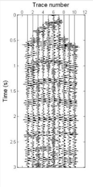
Before muting, in shot record 16, from 2.25 to 3 ms, trace 31 has an unusual, irregular trace. After muting, by muting the trace and interpolating it after, we managed to remove the bad trace entirely and replace it with a normal trace
a trace with abnormal amplitude exist in shot record 16 and it has been noticed that the bad trace is in trace 31. we zero the trace and interpolate the trace by averaging the properties from the neighbouring traces to remove anomaly and we replace the removed trace by normalized trace

Correction to Amplitude Losses
Among the various QC steps necessary to ultimately obtain an accurate seismic image of the subsurface structures is to correct for amplitude losses. There is a noticeable decreases in the amplitudes of its recorded traces with time as shows in Trace Editing figure (before muting).
Factors that lead to amplitude losses:
  • Transmission loss: This occurs at each geological reflector where part of the propagating seismic incident waves will be reflected, refracted, diffracted, scattered, etc. There is no loss here in terms of the mechanical energy since the lost energy merely travels somewhere else.
  • Geometric divergence: As the seismic wave spreads out from its source, its amplitude decays by an amount proportional to the reciprocal of the distance from the source to the location of the propagating seismic wave.
  • Absorption: This occurs where the seismic energy is converted into heat by friction. This loss is proportional to the exponential of the distance from the source.
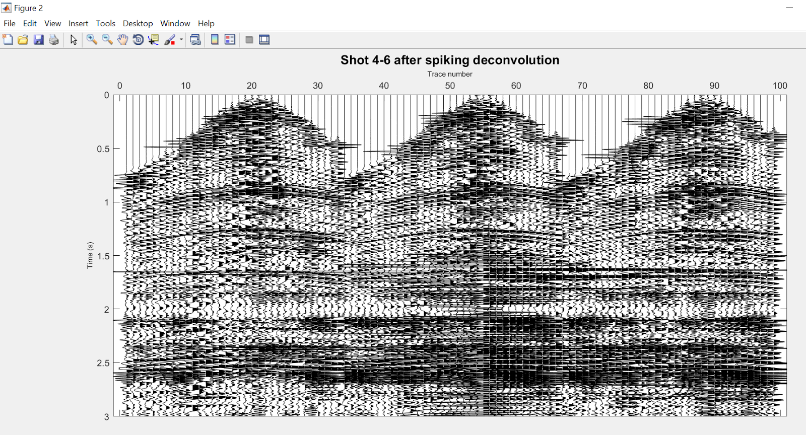
Amplitude correction is applied to seismic data sets a t various stage. Geometric divergence and absorption loss is corrected at pre-processing stage. The weak signal are being boost by adding more gain to the data. Figure below shows the amplitude enhancement gained on this shot gather. The figure below shows the seismic data shot gather number 8: before and after applying AGC method.
Objective : 
To compensate for amplitude losses due to transmission loss, geometric divergence and absorption.

...................................
%% Apply Gain
pow =2;
T=0;
Dg=iac(Dshot,t,pow,T);
Dgz=Dg;
%% Dsiplay data after apply gain
scale =1;
figure(2);
mwigb(Dg ,scale ,offset ,t)
xlabel('Offset(ft)','FontSize',14)
ylabel('Time(s)','FontSize',14)
title('Data after gain','FontSize',14)
%% Amplitude env gain
tnum=33;
seis_env_dB(Dshot,Dg,t,tnum)
seis_env_dB(Dshot,Dg,t)
%% Apply gain also
agc_gate =0.5;
T=1;
Dg1=AGCgain(Dshot,dt,agc_gate,T);
%% Dsiplay data after apply gain
scale=1;
figure(3);
mwigb(Dg1,scale ,offset ,t)
xlabel('Offset(ft)','FontSize',14)
ylabel('Time(s)','FontSize',14)
title('Data after gain','FontSize',14)
%% Also apply gain
agc_gate=0.5;
T=2;
Dg2=AGCgain(Dshot ,dt ,agc_gate ,T);
%% Dsiplay data after apply gain
scale=1;
figure(4);
mwigb(Dg2,scale ,offset ,t)
xlabel('Offset(ft)','FontSize',14)
ylabel('Time(s)','FontSize',14)
title('Data after gain','FontSize',16)
%%
clear D,clear Dg,clear Dshot,clear dt,clear dx,clear i,clear j
clear offset,clear p,clear pow,clear shot_num,clear t,clear T
save SeismicDataA_gain
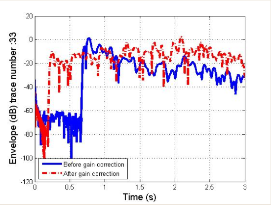
in shot record 33, the amplitude is concentrated in the shallower section only. The loss in amplitude towards the deeper section can be due to geometrical spreading,. After gain, the amplitude is balanced throughout the record length. 


blue line shows before gain, the average amplitude envelope the traces shows the \ decrease in amplitude over time.After gain (red line), we can observe the amplitude is more balanced .gain in deeper section can be observed .


  • RMS amplitude AGC: This method requires segmenting each trace into fixed time gates and then:
    • Calculate the RMS value in each gate.
    • Divide the desired RMS scaler by the RMS value of step 1 and multiply it by the amplitude of the sample at each gate center.
    • Interpolate between these gate centers and multiply the result by the amplitude of samples corresponding in time.
  • Instantaneous AGC: this is a bit different from the RMS AGC:
    • 1. Calculate the absolute mean value for in a given gate of length w.
    • 2. Divide the desired RMS scaler by the mean value of step 1 and multiply it by the amplitudes of all the samples in the gate.
    • 3. Slide the gate down by one sample and repeat steps 1-2 until you have calculated all the amplitudes of all trace samples that have been corrected.
The figure below shows the seismic data shot gather number  after applying the AGC using (a) instantaneous method (b) RMS method 

Computer Assignment
  • Shot gathers used in this computer assignment is shot gathers 11 till 14 as shows in the figure below.


  • Multiplication by a power of time and exponential gain function corrections with a,b = 1.8, 2.2 and 3.4 on the selected shot gathers. Then RMS AGC and instantaneous AGC method were applied on the same shot gathers.
Seismic data shot gather with a = 1.8, before and after applying amplitude correction gain method.


Seismic data with a= 1.8, shot gather after applying the AGC using the instantaneous and RMS based methods.
Seismic data shot gather with b = 1.8 before and after applying amplitude correction gain method.

DISCUSSION:


  AGC  method introduces an extreme amplitude gain at the bottom center. With increasing α, this noise is preserved while the upper reflection is greatly reduced. With exponential correction, most reflectors in the upper part are somehow diminished except in lower time window.However, increase in β also diminish lower reflectors.


CONCLUSION:

·        Quality control of seismic data is very crucial in the pre-processing of seismic data
·        AGC is an effective tool for gain control.
·        When conducting gain control, it is important to exclude extreme amplitude by trace editing so
       that it won’t be included in averaging process and to prevent masking the true reflectors.