lab 3:Seismic Noise Attenuation

Introduction :

Why is noise attenuation important?

1- Very simply, removal of the noise allows for all other signal processes to work more effectively. Deterministic processes, such as deriving surface consistent amplitude corrections or deconvolution operators, rely heavily on the quality of the input data. Many summation processes related specifically to dual sensor 'OBC' processing require calibration of the amplitude levels of each component for successful summation. This calibration cannot be correct in the presence of excessive noise..

2-Removal of the noise is a key component in preparing the data for pre-stack imaging. Common Depth Point (CDP) stack is obviously one of the most effective noise attenuation tools but not an option with pre-stack imaging. The noise must be addressed prior to imaging

3-Properly addressing the noise provides the opportunity to track amplitude anomalies and stratagraphic objectives with confidence.

4-Effective noise removal, which preserves the original amplitude and phase characteristics of the data, provides the opportunity for advanced attribute work and inversion to better understand the reservoir.

Seismic data are highly corrupted with noise or unwanted energy arising from different kinds of sources. This unwanted energy can be classified into two main categories: 

 * Random noise (incoherent noise). 

*  Coherent noise.  

Seismic data processing, in general, can never eliminate all noise contaminating the data. Hence, the objective of seismic data processing is to improve as much as possible the signal-to-noise ratio (SNR). 

2. SEISMIC SIGNAL & NOISE 

Noise in seismic records is variable in both time and space. Poor seismic records usually have SNR ratios less than one. One can define the signal of interest (coherent energy) as the energy which is coherent from trace to trace. Random noise, on the other hand, is the energy that is incoherent from trace to trace. Furthermore, data from seismic events is correlated and its energy is generally concentrated in a fairly narrow band of, while noise is more uncorrelated and broadband. However, this is only true for random noise. Spatially coherent noise is the most troublesome noise and can be highly correlated and sometimes aliased with the signal and. In general, noise can be considered as anything other than the desired signal. A more proper definition of noise contaminating seismic signals can be stated by defining the type of signals we are interested in. The authors in define the signal of interest as the energy that is most coherent and desirable for geophysical interpretation of primarily reflected arrivals (signals). Anything other than that is considered to be unwanted energy, i.e., noise. 

2.1 RANDOM NOISE

Disturbances in seismic data which lack phase coherency between adjacent traces are considered to be random noise. Unlike coherent noise energy, such energy is usually not related to the source that generates the seismic signals. In land seismic records, near-surface scatterers, wind, rain, and instrument are examples of sources generating random noise. Based on the assumption that random noise is an additive white Gaussian noise (AWGN), it can be attenuated easily in several different ways such as frequency filtering, deconvolution, wavelet denoising, filtering using Gabor representation, stacking and many other methods. As discussed before in Chapter 1, stacking usually suppresses most of the incoherent noise and, therefore, improves the SNR by a factor of √M, where M is equal to the number of stacked traces. 

2.2 COHERENT NOISE 

 coherent noise is the energy which is generated by the source. It is an undesirable energy that is added to the primary signals. Such energy shows consistent phase from trace to trace. Examples of such a type in land seismic records are: multiple reflections or multiples, surface waves like ground roll and, air waves, coherent scattered waves, dynamite ghosts, etc. Improper removal of coherent noise can affect nearly all the processing techniques and complicates interpretation of geological structures. There exist loads of techniques which deal with the problem of suppressing / attenuating coherent noise 

that contaminates seismic data. Since our real seismic data contains mainly ground roll coherent noise, its main characteristics will be described in the following subsection. 

OBJECTIVES:

• ·       To plot the magnitude spectra of shot gathers in frequency domain
•      To apply finite impulse response (FIR) and infinite impulse response (IIR) filter on shot
       gathers
•      To compare between the original data with applied filter data

PROCEDURE:

From this lab there were exist different means for such useful analysis: the frequency (or wave number) content of one-dimensional (1D) time (or space) signals, two-dimensional (2D) like the frequency-space (f−x) or the frequency-wave number (f−k) spectra; each of which can be used to obtain meaningful interpretation and, therefore, apply a suitable filtering technique. These plots and their corresponding analysis and interpretations are very useful, particularly, when applying linear filtering to 1D and/or 2D seismic data. You can use the following MATLAB m-file fx.m and fk.m (provided with the manual) to obtain the f−x and f−k magnitude spectra in dB.

clear,clc,close all
load SeismicDataA_gain
%%
shot_num=8:18;
p=0;
[Dshot,dt,dx,t,offset]=extracting_shots(Dgz,H,shot_num,p);
%%
scale=2;
mwigb(Dshot,scale,offset,t)
xlabel('Offset(ft)','FontSize',14)
ylabel('Time(s)','FontSize',14)
%%
[Data_f,f]=fx(Dshot,dt);
figure,
pcolor(offset,f,20*log10(fftshift(abs(Data_f),1)))
shading interp;
axis ij;
colormap(jet)
colorbar
xlabel('Offset(ft)','FontSize',14)
ylabel('Frequency (Hz)','FontSize',14)
set(gca,'xaxislocation','top')
axis([min(offset),max(offset),0,max(f)])
%%
[Data_fk,f,kx]=fk(Dshot,dt,dx);
figure,
pcolor(kx,f,20*log10(fftshift(abs(Data_fk))))
shading interp;
axis ij;
colormap(jet)
colorbar
xlabel('Wavenumber(1/ft)','FontSize',14)
ylabel('Frequency(Hz)','FontSize',14)
set(gca,'xaxislocation','top')
axis([min(kx),max(kx),0,max(f)])
%%
N=100;
cut_off=[15,60];
[Dbpf,Dbpf_f]=bpf_fir(Dshot,dt,N,cut_off);
save SeismicDataA_gain

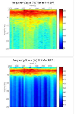
Figure above shows that shot gather 8 before and after applying the above mentioned BPF on each trace with the difference between both of them where clearly too great amount of the ground roll noise has been filtered

this figure also shows the f-x magnitude where the spectrum was banded between 15 and 60 Hz. Although frequency filtering like BFP has improved the data SNR by attenuating the ground roll noise, it has also lower the vertical resolution of the seismic data.

CONCLUSION:

• ·       The objectives are achieved.
•      High pass filter is useful to remove high frequency noise (ground roll).
•        Band pass filter is useful to remove noise while preserving reflectors.

​